ML Systems in Datacenters — LLM Inference Realities

Focus: TTFT vs. tokens/s, batching/latency, KV‑cache memory, PagedAttention/vLLM impact, practical serving tactics.

📋 Table of Contents

Serving KPIs & Phases (Prefill vs. Decode) — A Practical, No‑Assumptions Guide

Who this is for: Engineers and PMs who are new to LLM serving and want a solid, technically correct mental model that connects what you measure to what actually runs on the GPU.

1) The three metrics you'll see everywhere

1.1 Time to First Token (TTFT)

TTFT is the wall‑clock time from sending the request to the first byte/token arriving. It is dominated by the prefill phase (tokenization + network + scheduler queuing + the model's first pass).

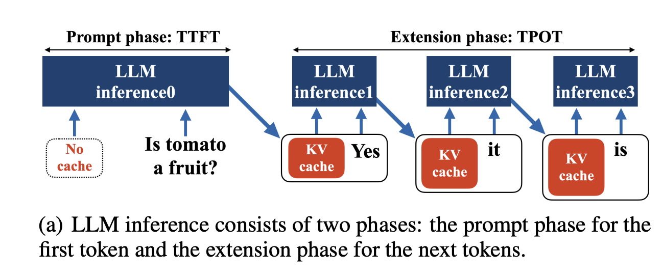Figure: LLM inference phases showing prefill (parallel processing) and decode (sequential generation). Source: Cho et al., "KV-Runahead: Scalable Causal LLM Inference by Parallel Key-Value Cache Generation"

Why it matters: users perceive responsiveness from TTFT; sub‑second TTFT dramatically improves UX for chat UIs and tools that stream output.

How people measure it: record a timestamp just before the request, then the timestamp when the first token is yielded. (Don't include model load time or cold starts unless that's part of your SLO.)

Understanding the Prefill Phase (and Why It Dominates TTFT)

This section gives you a visual, practical mental model for the prefill phase of LLM inference—the part that typically dominates TTFT. It includes ASCII diagrams, a timeline, and a concrete numeric example.

High‑Level Timeline

Time ──► | network & queue |=========== PREFILL (process full prompt) ===========| first token ► | decode t1 | decode t2 | decode t3 | …
           ↑——————————————— TTFT ————————————————↑

• TTFT is the wall‑clock time from when the request is sent until the first byte/token arrives.
• Prefill runs the entire prompt through the model, layer by layer, and writes per‑token K/V entries to the KV cache.
• Decode then generates output one token at a time, reusing the KV cache to avoid reprocessing the whole prompt.

Intuition: Prefill is compute‑bound (lots of matrix math across all prompt tokens), while decode tends to be memory/latency‑bound (small, per‑token steps that reuse the cache).

What the Model Does During Prefill

tokens → embeddings → [layer 1: self‑attn → MLP] → [layer 2 …] → … → logits
                         │                         │
                      write K,V to KV cache     write K,V to KV cache

• The model processes all prompt tokens in parallel per layer.
• Each attention layer stores keys/values (the KV cache) so the decode loop can reuse them.
• After prefill completes, the first token can be produced and streamed to the client.

Concrete (Illustrative) Example

The numbers below are hypothetical but realistic for a mid‑size modern decoder‑only LLM on a single data‑center GPU. Your exact figures will vary by hardware, batch size, scheduler, model, precision, and prompt length.

Scenario

• Prompt length: 1,000 tokens
• Output target: 100 tokens
• Network + queueing overhead: 50 ms
• Average prefill compute cost: 0.6 ms/token (aggregate across layers)
• Additional framework overhead: 50 ms
• Decode speed: 40 tokens/sec (~25 ms/token)

Derived timeline

• Prefill time ≈ 1,000 × 0.6 ms + 50 ms ≈ 650 ms
• TTFT ≈ 50 ms (net/queue) + 650 ms (prefill) ≈ 700 ms
• Decode time for 100 tokens ≈ 100 × 25 ms = 2,500 ms

Overall E2E (first token to last token): ~ 700 ms + 2,500 ms = 3.2 s

Timeline Visualization

Process Flow:

Why Prefill Often Dominates TTFT

• It must process every prompt token before any output can be streamed.
• Attention during prefill works over the whole prompt, so compute scales with prompt length.
• Techniques like chunked prefill, prefill–decode disaggregation, prefix caching, and KV‑Runahead/parallelization specifically target TTFT.

Practical Tips for Optimizing TTFT

• Keep prompts lean; move large context, tools, or retrieved content to structured inputs when possible.
• Use a serving stack that supports chunked prefill and balanced scheduling between compute‑bound prefill and memory‑bound decode.
• Measure TTFT separately from ITL/TPS to catch regressions specific to the prompt path.

1.2 Inter‑Token Latency (ITL) / Time‑Per‑Output‑Token (TPOT)

Once the first token appears, you care about the rate at which the rest of the tokens arrive. ITL (a.k.a. TPOT) is the average time between successive output tokens during decoding. Lower is better.

1.3 Tokens per Second (TPS, "tokens/s")

Throughput measured as output tokens per second (sometimes split into input and output token rates). Useful for capacity planning, autoscaling, and cost/performance tradeoffs. TPS must be considered alongside latency metrics—maximizing TPS alone can harm TTFT/ITL in interactive apps.

2) What actually happens on the GPU? Two phases

LLM inference alternates between two very different phases:

1. Prefill (a.k.a. prompt processing): the entire prompt (N tokens) is processed in parallel. This is compute‑bound (large GEMMs & attention) and mainly determines TTFT.
2. Decode (generation): one new token at a time. This stage repeatedly reads the KV cache created earlier. It's memory‑bandwidth/latency‑bound and mainly determines ITL/TPOT and tokens/s.

A first‑order mental model:

TTFT  ~=  tokenization + network + queueing + prefill compute
ITL   ~=  (KV-cache reads per step + small compute) / available memory bandwidth
TPS   ~=  1 / ITL   (for a single stream; scheduling affects multi‑stream TPS)

3) SLOs and tiers (how companies set expectations)

Most production systems define tiered SLOs:

• Premium / Low‑latency: tight TTFT (e.g., streaming begins quickly), controlled ITL for interactive tooling. May trade raw throughput for jitter control.
• Throughput tier / Batch: looser TTFT but very high TPS for offline or background workloads.
• Hybrid: separate budgets for TTFT vs. ITL, sometimes using disaggregation (see §5) to tune them independently.

4) Why prefill vs. decode behave so differently

• Prefill is parallel compute: big matrix multiplications over the whole prompt; very high arithmetic intensity. Scheduling and queuing can dominate here under load.
• Decode is memory traffic: each new token attends to all prior tokens by reading the stored K/V tensors (the KV cache). Arithmetic per token is small; latency is often gated by HBM bandwidth and cache locality.

This division is why optimizations often split along phase boundaries.

5) Scheduling and system patterns that move the needle

5.1 Continuous/rolling batching

Keep the GPUs saturated by continuously admitting new requests/tokens into active batches. This improves utilization and throughput without letting TTFT/ITL explode (good schedulers prioritize decodes).

5.2 Chunked prefill

Break large prefills into chunks that can be interleaved with decodes so decoders don't starve. Often combined with decode‑first prioritization to keep ITL stable.

5.3 Disaggregating prefill and decode

Run prefill and decode on different worker pools (or even different hardware/parallelism strategies). This lets you independently tune TTFT and ITL, and reduce tail latency interference when long prefills block decodes.

5.4 Prefix caching

If many requests share the same prompt prefix (system prompt, RAG boilerplate), reuse the KV cache for that prefix across requests and skip recompute. This reduces TTFT and pressure on memory capacity/bandwidth.

6) How to measure correctly (and avoid common pitfalls)

• Include queuing in TTFT if you're measuring end‑to‑end user latency.
• Stream responses to cut perceived latency; but remember that streaming does not change end‑to‑end latency for a fixed number of tokens. It mainly improves UX and early‑exit behavior.
• Separate metrics by phase in your dashboards: TTFT (prefill), ITL/TPOT (decode), plus request‑level p50/p95 and GPU‑level utilization/bandwidth counters.
• Watch prompt lengths: TTFT grows with input tokens; ITL grows mostly with output tokens and KV‑cache bandwidth pressure.
• Quantization and speculative decoding help both phases, but usually help prefill more than decode unless they reduce KV bandwidth demand too.

7) Quick checklist for first deployments

• Track TTFT, ITL/TPOT, TPS per route/model; alert on tail (p95/p99).
• Enable continuous batching; prefer decode‑first scheduling.
• Turn on chunked prefill for long prompts.
• Use prefix caching if prefixes repeat.
• Consider prefill/decode disaggregation when traffic & SLOs warrant it.
• Capacity plan with input token distribution and output length caps.

Further reading (annotated)

• NVIDIA: "Metrics for LLM benchmarking"—clear definitions of TTFT, ITL/TPOT and throughput, plus measurement tips.
• BentoML LLM Inference Handbook: concise explanations of prefill = compute‑bound, decode = memory‑bound, and why disaggregation helps.
• Databricks engineering blogs and docs: practical advice on balancing throughput vs. SLOs; evidence that decode is memory‑bound; how to benchmark.
• Microsoft "DéjàVu" paper: formalizes prefill compute‑bound vs. decode memory‑bound and discusses decode's near‑constant step time with KV cache.
• vLLM docs: continuous batching, chunked prefill, and prefix caching knobs you can use today.

Additional Prefill & TTFT Optimization Resources

• vLLM – Optimization & Tuning (Chunked Prefill): https://docs.vllm.ai/en/stable/configuration/optimization.html
• NVIDIA – TensorRT‑LLM: Chunked Prefill (developer blog): https://developer.nvidia.com/blog/streamlining-ai-inference-performance-and-deployment-with-nvidia-tensorrt-llm-chunked-prefill/
• Apple ML Research – KV‑Runahead (parallelizing the prompt phase to reduce TTFT): https://machinelearning.apple.com/research/kv-runahead (arXiv: https://arxiv.org/html/2405.05329)
• LLM Inference Handbook – Prefill/Decode overview & disaggregation: https://bentoml.com/llm/inference-optimization/prefill-decode-disaggregation
• Glean – How KV caches impact Time‑to‑First‑Token (charts & practical notes): https://www.glean.com/jp/blog/glean-kv-caches-llm-latency

These links contain diagrams and deeper explanations of the prefill → first token → decode flow, plus techniques to improve TTFT.

(See the chat message for live citation links.)

8) KV‑Cache Sizing, Pressure & PagedAttention — From First Principles

Goal: Understand exactly what the KV cache is, how to size it, where memory is wasted, and why systems like vLLM with PagedAttention fix the problem. This section assumes no prior GPU background.

8.1) What is the KV cache?

During attention, every token produces three vectors per layer: Q, K, and V.
For decoding the next token, the model only needs the new Q—but it must read all prior K and V for that sequence (and head) to compute attention. We therefore store all previously computed K/V in GPU memory as the KV cache so we don't recompute them at every step.

Implication: decode steps are read‑heavy on the KV cache, so bandwidth/latency dominate performance once generation begins.

8.2) How big is the KV cache? (Exact formula + example)

For most decoder‑only transformers, the KV memory for one sequence of length T is approximately:

KV_bytes_per_sequence  ≈  T × L × H × D × 2 × bytes_per_elem

Where:

• T = tokens processed so far (context length)
• L = number of transformer layers
• H = attention heads
• D = head dimension
• The factor 2 accounts for K and V (no Q is stored)
• bytes_per_elem = 2 for FP16/BF16, 1 for FP8/INT8 variants, 4 for FP32

For a batch of B sequences, multiply by B (or by the sum of individual sequence lengths).

Worked example (matches the slide)

Batch = 16, Layers = 32, Heads = 32, Head dim = 128, Precision = FP16 (2 bytes), Context = 4096 tokens:

KV_bytes ≈ 16 × 32 × 32 × 128 × 2 × 2 × 4096
         = 34.36 GB  (decimal)  = 32.00 GiB (binary)

That is just for KV — you still need memory for activations, parameters, and workspace. This is why naïve serving often "runs out of VRAM" even on large GPUs.

8.3) Why naïve allocation wastes memory (fragmentation)

If you allocate one contiguous slab per request sized to the max context (or grow and copy it as context expands), three bad things happen:

1. External fragmentation: small holes between slabs can't be used for new sequences.
2. Internal fragmentation: you reserve space for max length even if the sequence is short.
3. Resize stalls: when a request outgrows its slab, you may need to reallocate/copy, which stalls decoding.

These pathologies cap batch size and increase tail latency.

8.4) PagedAttention: make KV look like virtual memory

Key idea: manage KV in fixed‑size blocks (e.g., 16–32 tokens per block) and maintain a page table that maps each sequence's logical blocks to physical blocks located anywhere in GPU memory.

Benefits:

• Near‑zero external fragmentation: any free block can be reused for any sequence.
• Small internal fragmentation: at most one partial block per sequence.
• Fast growth: append a block; no copy of prior KV.
• Sharing & caching: identical prefixes across requests can point to the same physical blocks (prefix caching).
• Kernel‑aware: attention kernels are optimized to fetch from these paged KV layouts efficiently.

You'll see knobs like block_size = 16 or 32 tokens and features like automatic prefix caching in modern systems (e.g., vLLM).

8.5) Practical knobs that relieve KV pressure

• Reduce precision for KV (e.g., FP8/INT8) to cut bytes per element.
• Prefix caching to avoid recomputing shared prompts; the reused blocks do not multiply memory.
• Continuous batching to keep utilization high while admitting decodes promptly.
• Chunked prefill so long prompts don't starve decoders.
• KV compression/eviction (research): e.g., SnapKV, RocketKV, head/token dropping—trade a bit of model quality for much lower bandwidth/VRAM.
• Disaggregate prefill & decode so memory‑bound decode runs on appropriately tuned instances without being interrupted by long prefills.

8.6) Sanity‑check calculator (how to size a box)

Given model {L, H, D} and precision p:

KV bytes per token  = 2 × L × (H × D) × bytes(p)
KV bytes per seq    = (tokens_so_far) × [bytes per token]
KV bytes per batch  = sum_over_sequences(KV bytes per seq)

Add headroom for: model weights, temporary activations (prefill), CUDA workspace, attention metadata, and fragmentation. For multi‑tenant services, assume p95 input lengths, not just means.

8.7) What this looks like in a real engine (vLLM)

• PagedAttention kernels read KV from block‑structured caches and use a page‑table lookup to hop to the right physical blocks efficiently.
• Block management shows up in configs (block_size), schedulers (preempt & resume sequences across blocks), and features like automatic prefix caching and continuous batching.
• Chunked prefill is enabled by default in newer vLLM releases so decodes keep flowing even under long prefills.

8.8) Takeaways

• KV footprint scales with B × T × L × H × D × precision—it grows linearly with context length and batch size.
• Decode performance is often capped by memory bandwidth to read KV—optimize for locality, precision, and block layout.
• PagedAttention plus prefix caching and continuous batching are practical, production‑proven ways to reduce waste and improve both latency and throughput.

Further reading (annotated)

• NVIDIA "Mastering LLM Techniques – Inference Optimization": includes the canonical KV sizing formula and concrete examples.
• vLLM paper & docs on PagedAttention and block‑level memory management; slides detailing block sizes (16/32 tokens) and how page tables minimize fragmentation.
• vLLM design docs for paged attention kernels and prefix caching.
• Research on KV compression & bandwidth reduction (e.g., RocketKV, head‑level compression).

9) Scheduling/batching policies

• Static batching: good throughput, hurts idling and tail latency.
• Continuous batching: join in‑flight batches between tokens; better balance.
• Speculative decoding: draft model proposes k tokens, target verifies; reduces wall time under accuracy guardrails.
• Separate low‑latency tier (small batches, reserved capacity) from throughput tier (large batches).

10) Practical engineering checklist

• Profile prefill vs. decode separately; scale resources accordingly (more tensor cores vs. more KV BW).
• Keep KV in HBM; if offloading to CPU, prefetch and overlap DMA; pin pages; use large IOMMU pages.
• Use quantization (int8/int4) where quality allows; beware quantization‑aware kernels for attention.
• Consider MIG or node‑level isolation; noisy neighbors wreak havoc on tails.
• Instrument TTFT distribution and tokens/s per request; log batch sizes and effective context lengths.

11) Debugging playbook

• TTFT spikes: request coalescing delays, tokenizer CPU hotspot, cold model weights, page faults.
• Low tokens/s: poor achieved occupancy, unfused attention kernels, KV gather patterns causing bank conflicts or L2 thrash, PCIe back‑pressure.
• OOM: reduce max context or enable paged KV, apply prefix caching, share LoRA adapters.

12) Capacity planning sketch (worked)

Target p99 ≤ 300 ms for 128‑token responses. Budget: TTFT 50 ms, decode 250 ms.
If decode cost/token ≈ 0.5 ms at batch=32 ⇒ tokens/s/GPU ≈ 2000.
With continuous batching + paged KV, expect +20–50% throughput depending on context distribution; validate on your model mix.

References

• vLLM PagedAttention; NVIDIA TensorRT‑LLM KV manager; CUDA performance backgrounders.