Stable Diffusion vs ViT (Vision Transformer)
Technical comparison of Vision Transformer and Stable Diffusion architectures and their convergence.
Prerequisites
Make sure you're familiar with these concepts before diving in:
Learning Objectives
By the end of this topic, you will be able to:
Table of Contents
Vision Transformer vs Stable Diffusion: Comprehensive Technical Documentation
Table of Contents
- Executive Summary
- Technology Overview
- Architectural Analysis
- Core Components Comparison
- Use Cases and Applications
- Performance Characteristics
- Implementation Considerations
- Recent Convergence: Diffusion Transformers
- Practical Deployment Guide
- Future Roadmap
- Decision Framework
- Conclusion
1. Executive Summary
1.1 Quick Comparison Matrix
| Aspect | Vision Transformer (ViT) | Stable Diffusion |
|---|---|---|
| PRIMARY FUNCTION | Image Understanding/Classification | Image Generation from Text |
| ARCHITECTURE TYPE | Pure Transformer | Hybrid (U-Net + VAE + CLIP) |
| INPUT | Raw Images | Text Prompts + Noise |
| OUTPUT | Class Labels/Features | Generated Images |
| TRAINING PARADIGM | Supervised Learning | Diffusion Process |
| COMPUTATIONAL FOCUS | Discriminative Tasks | Generative Tasks |
| MODEL SIZE | 86M - 632M parameters | 860M - 6.6B parameters |
| INFERENCE SPEED | Fast (single forward pass) | Slow (multiple denoising steps) |
| DATA REQUIREMENTS | Large labeled datasets | Large image-text pairs |
1.2 Key Insight
While initially designed for different purposes, these technologies are converging through Diffusion Transformers (DiT), which replace Stable Diffusion's U-Net with transformer architectures inspired by ViT.
2. Technology Overview
2.1 Vision Transformer (ViT)
Purpose: Revolutionize computer vision by applying transformer architecture directly to images.
Core Innovation: Treats images as sequences of patches, eliminating the need for convolutional layers in image classification.
Key Principle:
"An image is worth 16x16 words" - Each 16×16 patch becomes a token processed by self-attention.
Architecture Philosophy:
- Minimal inductive bias
- Global receptive field from first layer
- Scalable with data and compute
2.2 Stable Diffusion
Purpose: Generate high-quality images from textual descriptions using diffusion processes.
Core Innovation: Combines latent diffusion with cross-attention conditioning for efficient text-to-image generation.
Key Principle:
Progressive denoising in latent space with text guidance produces photorealistic images.
Architecture Philosophy:
- Multi-modal conditioning
- Latent space efficiency
- Iterative refinement process
3. Architectural Analysis
3.1 Vision Transformer Architecture
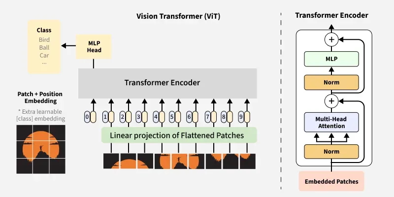
Figure 1: Vision Transformer (ViT) Architecture Overview - Complete pipeline from image patch embedding through transformer encoder layers to classification output
Source: GeeksforGeeks - Vision Transformer (ViT) Architecture
Input Processing Pipeline:
┌─────────────────┐    ┌──────────────────┐    ┌─────────────────┐
│   Image Input   │ -> │  Patch Embedding │ -> │ Position Embed  │
│   (224×224×3)   │    │   (196 patches)  │    │   + [CLS] Token │
└─────────────────┘    └──────────────────┘    └─────────────────┘
                                ↓
┌─────────────────┐    ┌──────────────────┐    ┌─────────────────┐
│ Classification  │ <- │  Transformer     │ <- │  Input Sequence │
│     Head        │    │  Encoder (12×)   │    │  (197 tokens)   │
└─────────────────┘    └──────────────────┘    └─────────────────┘
3.1.1 Detailed Component Breakdown:
1. Patch Embedding Layer
class PatchEmbedding(nn.Module):
    def __init__(self, img_size=224, patch_size=16, in_channels=3, embed_dim=768):
        super().__init__()
        self.num_patches = (img_size // patch_size) ** 2
        self.projection = nn.Conv2d(in_channels, embed_dim,
                                   kernel_size=patch_size, stride=patch_size)

    def forward(self, x):
        # x: [B, C, H, W] -> [B, num_patches, embed_dim]
        x = self.projection(x).flatten(2).transpose(1, 2)
        return x
2. Multi-Head Self-Attention
# Each patch attends to all other patches globally
attention_weights = softmax(Q @ K.T / sqrt(d_k)) @ V
3. Position Encoding
- Learnable 1D position embeddings
- Encodes spatial relationships between patches
- Added to patch embeddings before transformer processing
3.2 Stable Diffusion Architecture
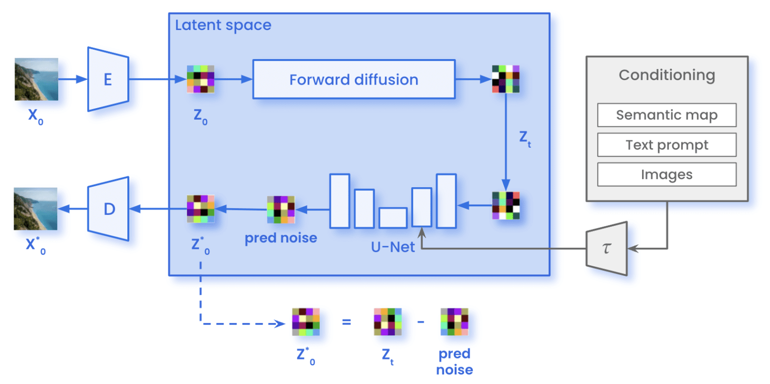
Figure 3a: Stable Diffusion Training Architecture - Complete training pipeline showing latent space operations, forward diffusion process, U-Net denoising network, and noise prediction loss calculation
Source: Marvik.ai - An Introduction to Diffusion Models and Stable Diffusion
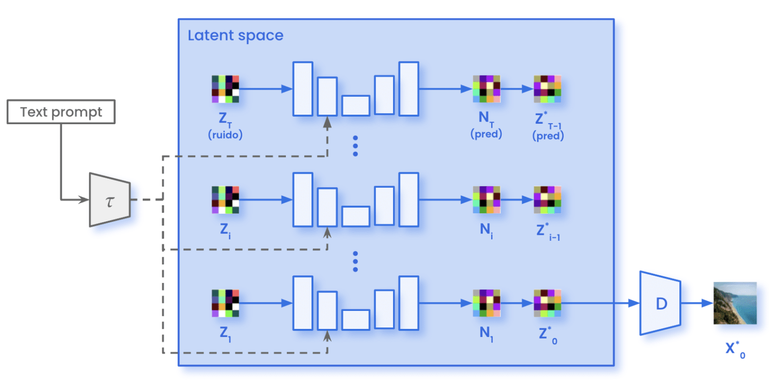
Figure 3b: Stable Diffusion Sampling Architecture - Inference pipeline demonstrating iterative denoising process in latent space with text conditioning for image generation
Source: Marvik.ai - An Introduction to Diffusion Models and Stable Diffusion
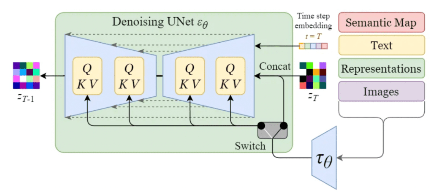
Figure 3c: U-Net Cross-Attention Conditioning Mechanism - Detailed view of how text embeddings condition the denoising process through cross-attention layers (Q/K/V) with timestep and semantic conditioning
Source: Marvik.ai - An Introduction to Diffusion Models and Stable Diffusion
Text-to-Image Generation Pipeline:
┌─────────────────┐    ┌──────────────────┐    ┌─────────────────┐
│   Text Prompt   │ -> │  CLIP Text       │ -> │  Text Embedding │
│ "A red bicycle" │    │  Encoder         │    │   (77×768)      │
└─────────────────┘    └──────────────────┘    └─────────────────┘
                                                        ↓
┌─────────────────┐    ┌──────────────────┐    ┌─────────────────┐
│  Generated      │ <- │      VAE         │ <- │     U-Net       │
│     Image       │    │    Decoder       │    │   Denoising     │
│   (512×512×3)   │    │                  │    │   Process       │
└─────────────────┘    └──────────────────┘    └─────────────────┘
                                                        ↑
                              ┌─────────────────────────┘
                              │
                    ┌─────────────────┐
                    │  Random Noise   │
                    │    Latent       │
                    │   (64×64×4)     │
                    └─────────────────┘
3.2.1 Detailed Component Breakdown:
1. CLIP Text Encoder
# Transformer-based text encoder
text_embeddings = clip_text_encoder(tokenized_text)
# Output: [batch_size, 77, 768]
2. U-Net Architecture
The U-Net serves as the core denoising component in Stable Diffusion, responsible for iteratively removing noise from latent representations while being conditioned on text embeddings. Originally designed for biomedical image segmentation, U-Net's symmetric encoder-decoder architecture with skip connections makes it exceptionally well-suited for diffusion processes.
class UNet2DConditionModel:
    def __init__(self):
        self.down_blocks = nn.ModuleList([...])  # Encoder
        self.mid_block = UNetMidBlock2DCrossAttn(...)  # Bottleneck
        self.up_blocks = nn.ModuleList([...])    # Decoder

    def forward(self, latent, timestep, text_embedding):
        # Cross-attention between image and text features
        return denoised_latent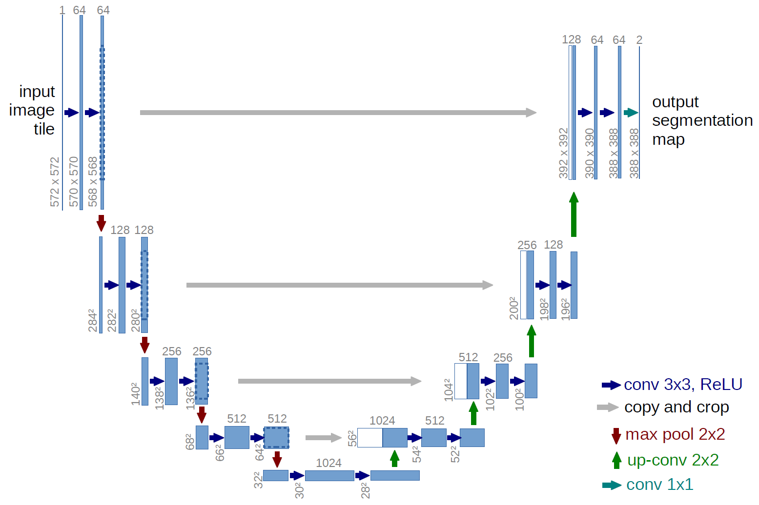
Figure 2: U-Net Architecture with Skip Connections - Encoder-decoder structure enabling precise noise prediction in diffusion models through multi-scale feature processing
Source: Ronneberger et al. - U-Net: Convolutional Networks for Biomedical Image Segmentation (2015)
3.2.2 Key Architectural Components:
Encoder (Contracting Path):
- Series of convolutional blocks with downsampling
- Captures context through progressively larger receptive fields
- Feature maps: 64 → 128 → 256 → 512 → 1024 channels
- Each step reduces spatial resolution by 2×
Decoder (Expanding Path):
- Mirror structure of encoder with upsampling
- Combines low-level and high-level features
- Gradual spatial resolution recovery: 1024 → 512 → 256 → 128 → 64 channels
- Transpose convolutions for learned upsampling
Skip Connections:
- Direct pathways from encoder to corresponding decoder layers
- Preserves fine-grained spatial information lost during downsampling
- Enables precise localization essential for noise prediction
- Concatenation of encoder features with decoder features
Cross-Attention Integration (Stable Diffusion Enhancement):
- Text conditioning through cross-attention layers
- Query from image features, Key/Value from text embeddings
- Enables semantic guidance during denoising process
- Multiple attention heads for diverse conditioning patterns
3.2.3 Timestep Conditioning:
The U-Net receives timestep embeddings to understand the current noise level:
def timestep_embedding(timesteps, dim):
    """Sinusoidal timestep embeddings"""
    half = dim // 2
    freqs = torch.exp(-math.log(10000) * torch.arange(half) / half)
    args = timesteps[:, None] * freqs[None, :]
    embedding = torch.cat([torch.cos(args), torch.sin(args)], dim=-1)
    return embedding
This architectural design enables the U-Net to:
- Maintain spatial coherence through skip connections
- Process multi-scale features via encoder-decoder structure
- Integrate semantic guidance through cross-attention
- Handle variable noise levels via timestep conditioning
3. VAE (Variational Autoencoder)
# Encode image to latent space (8× compression)
latent = vae.encode(image).latent_dist.sample() * 0.18215

# Decode latent back to image space
image = vae.decode(latent / 0.18215).sample
4. Core Components Comparison
4.1 Attention Mechanisms
4.1.1 Vision Transformer: Self-Attention
Purpose: Enable each patch to attend to all other patches
Mechanism:
# Global self-attention across all patches
Q = patches @ W_q  # Query matrix
K = patches @ W_k  # Key matrix
V = patches @ W_v  # Value matrix

attention = softmax(Q @ K.T / sqrt(d_k)) @ VCharacteristics:
- Symmetric attention (bidirectional)
- Global receptive field
- Computational complexity: O(n²)
- Learns spatial relationships implicitly
4.1.2 Stable Diffusion: Cross-Attention
Purpose: Condition image generation on text descriptions
Mechanism:
# Cross-attention between image features and text embeddings
Q = image_features @ W_q     # Query from image
K = text_embeddings @ W_k    # Key from text
V = text_embeddings @ W_v    # Value from text

cross_attention = softmax(Q @ K.T / sqrt(d_k)) @ VCharacteristics:
- Asymmetric attention (unidirectional)
- Multi-modal conditioning
- Enables semantic control
- Different modalities interaction
4.2 Input Processing
4.2.1 Vision Transformer: Patch Tokenization
def process_input(image):
    # Step 1: Divide into patches
    patches = image.unfold(dimension=2, size=16, step=16)
                  .unfold(dimension=3, size=16, step=16)

    # Step 2: Flatten patches
    flattened = patches.reshape(batch_size, num_patches, -1)

    # Step 3: Linear projection
    tokens = linear_projection(flattened)

    # Step 4: Add position embeddings
    tokens += position_embeddings

    return tokens
4.2.2 Stable Diffusion: Multi-Modal Processing
def process_inputs(text_prompt, noise_latent, timestep):
    # Text processing
    text_tokens = tokenizer(text_prompt)
    text_embeddings = clip_text_encoder(text_tokens)

    # Noise timestep embedding
    time_embedding = timestep_embedding(timestep)

    # Latent preparation
    noisy_latent = add_noise(clean_latent, noise, timestep)

    return text_embeddings, noisy_latent, time_embedding
4.3 Training Objectives
4.3.1 Vision Transformer: Classification Loss
def training_objective(model, images, labels):
    # Forward pass
    patch_embeddings = patch_embed(images)
    features = transformer_encoder(patch_embeddings)
    cls_token = features[:, 0]  # CLS token representation
    logits = classification_head(cls_token)

    # Cross-entropy loss
    loss = cross_entropy(logits, labels)
    return loss
4.3.2 Stable Diffusion: Noise Prediction Loss
def training_objective(model, images, text_embeddings):
    # Add noise to images
    noise = torch.randn_like(images)
    timesteps = torch.randint(0, 1000, (batch_size,))
    noisy_images = add_noise(images, noise, timesteps)

    # Predict noise
    predicted_noise = model(noisy_images, timesteps, text_embeddings)

    # MSE loss between predicted and actual noise
    loss = mse_loss(predicted_noise, noise)
    return loss
5. Use Cases and Applications
5.1 Vision Transformer Applications
5.1.1 Primary Use Cases:
-
Image Classification
- ImageNet classification
- Fine-grained categorization
- Medical image diagnosis
-
Feature Extraction
- Transfer learning backbone
- Representation learning
- Similarity search
-
Dense Prediction Tasks (with modifications)
- Object detection (DETR)
- Semantic segmentation (SETR)
- Instance segmentation
5.1.2 Industry Applications:
Healthcare:
- Medical imaging analysis
- Pathology slide classification
- Radiology report automation

Autonomous Vehicles:
- Scene understanding
- Traffic sign recognition
- Pedestrian detection

E-commerce:
- Product categorization
- Visual search
- Quality assessment

Manufacturing:
- Defect detection
- Quality control
- Assembly verification
5.2 Stable Diffusion Applications
5.2.1 Primary Use Cases:
-
Creative Content Generation
- Art and illustration creation
- Concept art for games/movies
- Marketing materials
-
Image Editing and Enhancement
- Inpainting (filling missing regions)
- Super-resolution
- Style transfer
-
Data Augmentation
- Synthetic dataset generation
- Rare case simulation
- Privacy-preserving data
5.2.2 Industry Applications:
Media & Entertainment:
- Movie concept art
- Game asset creation
- Advertising visuals

Fashion & Design:
- Product visualization
- Pattern generation
- Virtual try-on

Architecture:
- Building visualization
- Interior design
- Landscape planning

Education:
- Textbook illustrations
- Historical reconstructions
- Scientific visualizations
6. Performance Characteristics
6.1 Computational Requirements
6.1.1 Vision Transformer
Training Requirements:
Model: ViT-Base/16
Parameters: 86M
Training Data: ImageNet-21k (14M images)
Hardware: 8× V100 GPUs
Training Time: ~3 days
Memory: ~32GB per GPU
Inference Performance:
Input Size: 224×224×3
Latency: ~5ms (V100)
Throughput: ~2000 images/second
Memory: ~2GB
Power: ~300W
6.1.2 Stable Diffusion
Training Requirements:
Model: Stable Diffusion v1.5
Parameters: 860M (total pipeline)
Training Data: LAION-5B subset
Hardware: Multiple A100 clusters
Training Time: Several weeks
Memory: ~40GB per GPU
Inference Performance:
Input: Text prompt
Output Size: 512×512×3
Latency: ~3-10 seconds (50 steps)
Memory: ~8-12GB
Power: ~300W
Batch Processing: Limited by memory
6.2 Scalability Analysis
6.2.1 Vision Transformer Scaling Laws
# Performance scales with:
# 1. Model size (parameters)
# 2. Dataset size
# 3. Compute budget

performance ∝ log(parameters) × log(data_size) × log(compute)

# Scaling trends:
ViT-Base:   86M params  -> 81.8% ImageNet accuracy
ViT-Large:  307M params -> 85.2% ImageNet accuracy
ViT-Huge:   632M params -> 88.5% ImageNet accuracy
6.2.2 Stable Diffusion Scaling Laws
# Quality scales with:
# 1. Model parameters
# 2. Training steps
# 3. Data diversity

quality ∝ log(parameters) × log(training_steps) × log(data_diversity)

# Recent scaling examples:
SD v1.5:    860M params  -> High quality 512×512
SD v2.1:    865M params  -> Improved 768×768
SDXL:       3.5B params  -> Superior 1024×1024
6.3 Memory and Efficiency
6.3.1 Vision Transformer Efficiency
def vit_memory_analysis():
    """Memory breakdown for ViT-Base inference"""

    input_image = 224 * 224 * 3 * 4  # 0.6MB (float32)
    patch_embeddings = 196 * 768 * 4  # 0.6MB
    attention_weights = 12 * 12 * 196 * 196 * 4  # 221MB
    intermediate_activations = 196 * 3072 * 4  # 2.4MB

    total_memory = 225MB  # Approximate
    return total_memory
6.3.2 Stable Diffusion Efficiency
def sd_memory_analysis():
    """Memory breakdown for Stable Diffusion inference"""

    text_encoder = 123M * 4  # 492MB
    unet_model = 860M * 4   # 3.4GB
    vae_model = 84M * 4     # 336MB
    latent_space = 64 * 64 * 4 * 4  # 65KB
    attention_maps = 1000MB  # Variable

    total_memory = ~6GB  # Approximate
    return total_memory
7. Implementation Considerations
7.1 Vision Transformer Implementation
7.1.1 Prerequisites and Setup
# Required libraries
import torch
import torch.nn as nn
import torchvision.transforms as transforms
from timm import create_model  # PyTorch Image Models

# Model initialization
model = create_model('vit_base_patch16_224', pretrained=True)
model.eval()

# Input preprocessing
transform = transforms.Compose([
    transforms.Resize((224, 224)),
    transforms.ToTensor(),
    transforms.Normalize(mean=[0.485, 0.456, 0.406],
                        std=[0.229, 0.224, 0.225])
])
7.1.2 Training Configuration
# Training hyperparameters
config = {
    'learning_rate': 3e-4,
    'batch_size': 512,
    'epochs': 300,
    'weight_decay': 0.3,
    'warmup_epochs': 10,
    'optimizer': 'AdamW',
    'scheduler': 'cosine',
    'augmentation': 'RandAugment',
    'mixup_alpha': 0.8,
    'cutmix_alpha': 1.0,
    'label_smoothing': 0.1
}
7.1.3 Fine-tuning Best Practices
def fine_tune_vit(model, num_classes, learning_rate=1e-4):
    # Freeze backbone layers
    for param in model.parameters():
        param.requires_grad = False

    # Replace classification head
    model.head = nn.Linear(model.head.in_features, num_classes)

    # Unfreeze last few layers for fine-tuning
    for param in model.blocks[-2:].parameters():
        param.requires_grad = True

    # Use lower learning rate for fine-tuning
    optimizer = torch.optim.AdamW([
        {'params': model.head.parameters(), 'lr': learning_rate},
        {'params': model.blocks[-2:].parameters(), 'lr': learning_rate * 0.1}
    ])

    return model, optimizer
7.2 Stable Diffusion Implementation
7.2.1 Prerequisites and Setup
# Required libraries
import torch
from diffusers import StableDiffusionPipeline, DDIMScheduler
from transformers import CLIPTextModel, CLIPTokenizer

# Pipeline initialization
pipe = StableDiffusionPipeline.from_pretrained(
    "runwayml/stable-diffusion-v1-5",
    torch_dtype=torch.float16,
    safety_checker=None,
    requires_safety_checker=False
)
pipe = pipe.to("cuda")
7.2.2 Generation Configuration
# Generation parameters
generation_config = {
    'num_inference_steps': 50,
    'guidance_scale': 7.5,
    'height': 512,
    'width': 512,
    'generator': torch.Generator().manual_seed(42),
    'negative_prompt': "blurry, low quality, distorted"
}

# Generate image
image = pipe(
    prompt="A serene landscape with mountains and lake",
    **generation_config
).images[0]
7.2.3 Custom Pipeline Development
class CustomStableDiffusion:
    def __init__(self, model_path):
        self.vae = AutoencoderKL.from_pretrained(model_path, subfolder="vae")
        self.tokenizer = CLIPTokenizer.from_pretrained(model_path, subfolder="tokenizer")
        self.text_encoder = CLIPTextModel.from_pretrained(model_path, subfolder="text_encoder")
        self.unet = UNet2DConditionModel.from_pretrained(model_path, subfolder="unet")
        self.scheduler = DDIMScheduler.from_pretrained(model_path, subfolder="scheduler")

    def generate(self, prompt, num_steps=50):
        # Encode text
        text_inputs = self.tokenizer(prompt, return_tensors="pt")
        text_embeddings = self.text_encoder(text_inputs.input_ids)[0]

        # Initialize random latent
        latent = torch.randn(1, 4, 64, 64)

        # Denoising loop
        self.scheduler.set_timesteps(num_steps)
        for timestep in self.scheduler.timesteps:
            noise_pred = self.unet(latent, timestep, text_embeddings).sample
            latent = self.scheduler.step(noise_pred, timestep, latent).prev_sample

        # Decode to image
        image = self.vae.decode(latent).sample
        return image
8. Recent Convergence: Diffusion Transformers
8.1 The Paradigm Shift
The computer vision field is witnessing a significant convergence between ViT and diffusion models through Diffusion Transformers (DiT), which replace the U-Net backbone in diffusion models with transformer architectures.
8.2 DiT Architecture Analysis
8.2.1 Core Innovation
class DiffusionTransformer(nn.Module):
    def __init__(self, input_size=32, patch_size=2, in_channels=4,
                 hidden_size=1152, depth=28, num_heads=16):
        super().__init__()
        self.patch_embed = PatchEmbed(input_size, patch_size, in_channels, hidden_size)
        self.pos_embed = nn.Parameter(torch.zeros(1, num_patches, hidden_size))

        # Transformer blocks with adaptive layer norm
        self.blocks = nn.ModuleList([
            DiTBlock(hidden_size, num_heads) for _ in range(depth)
        ])

        # Final layer for noise prediction
        self.final_layer = FinalLayer(hidden_size, patch_size, out_channels)

    def forward(self, x, t, y):
        """
        x: Noisy latent patches
        t: Timestep embedding
        y: Class label embedding
        """
        x = self.patch_embed(x) + self.pos_embed

        for block in self.blocks:
            x = block(x, t, y)  # Condition on timestep and class

        x = self.final_layer(x, t)
        return x
8.2.2 Key Improvements Over U-Net
1. Scalability
# DiT scaling results (ImageNet 256×256)
models = {
    'DiT-S/2': {'params': '33M', 'FID': 5.02},
    'DiT-B/2': {'params': '130M', 'FID': 3.04},
    'DiT-L/2': {'params': '458M', 'FID': 2.55},
    'DiT-XL/2': {'params': '675M', 'FID': 2.27}  # SOTA
}

# Clear scaling trend: larger models → better FID scores
2. Adaptive Layer Normalization
class AdaLN(nn.Module):
    """Adaptive Layer Normalization conditioned on timestep and class"""
    def __init__(self, hidden_size, conditioning_size):
        super().__init__()
        self.ln = nn.LayerNorm(hidden_size, elementwise_affine=False)
        self.linear = nn.Linear(conditioning_size, 2 * hidden_size)

    def forward(self, x, conditioning):
        scale, shift = self.linear(conditioning).chunk(2, dim=-1)
        return self.ln(x) * (1 + scale) + shift
3. Global Attention vs Local Convolutions
# U-Net: Local receptive field
conv_layer = nn.Conv2d(in_channels, out_channels, kernel_size=3)

# DiT: Global receptive field
attention_layer = MultiHeadAttention(embed_dim, num_heads)
8.3 Stable Diffusion 3.0 Integration
Recent Stable Diffusion 3.0 models have adopted transformer-based architectures:
# SD3 Architecture (Simplified)
class SD3DiffusionTransformer:
    def __init__(self):
        self.joint_transformer = MultiModalDiT(
            text_dim=4096,
            image_dim=1536,
            depth=24,
            heads=24
        )

    def forward(self, image_latents, text_embeddings, timestep):
        # Joint attention between image and text
        joint_features = torch.cat([image_latents, text_embeddings], dim=1)

        # Process with transformer
        output = self.joint_transformer(joint_features, timestep)

        # Split back to image predictions
        image_output = output[:, :image_latents.shape[1]]
        return image_output
8.4 Performance Comparison: DiT vs U-Net
| Model Type | Parameters | FID (ImageNet 256) | Training Time | Inference Speed |
|---|---|---|---|---|
| U-Net (LDM) | 400M | 3.60 | 7 days | 2.5s |
| DiT-L/2 | 458M | 2.55 ↓ | 7 days | 2.8s |
| DiT-XL/2 | 675M | 2.27 ↓↓ | 10 days | 3.2s |
8.5 Hybrid Approaches
8.5.1 CoAtNet: Convolution + Attention
class CoAtNet(nn.Module):
    """Combines convolutional and attention mechanisms"""
    def __init__(self):
        super().__init__()
        # Early layers: Convolution for local features
        self.conv_stem = ConvStem()
        self.conv_stages = nn.ModuleList([ConvBlock() for _ in range(2)])

        # Later layers: Attention for global features
        self.attn_stages = nn.ModuleList([AttnBlock() for _ in range(2)])

    def forward(self, x):
        # Convolutional processing
        for conv_block in self.conv_stages:
            x = conv_block(x)

        # Attention processing
        for attn_block in self.attn_stages:
            x = attn_block(x)

        return x
9. Practical Deployment Guide
9.1 Vision Transformer Deployment
9.1.1 Model Selection Guidelines
def select_vit_model(use_case, data_size, compute_budget):
    """Guide for selecting appropriate ViT variant"""

    if use_case == "mobile_deployment":
        return "Mobile-ViT" if compute_budget == "low" else "DeiT-Small"

    elif data_size < 100000:  # Small dataset
        return "ViT-Base/16 (pre-trained)"

    elif data_size < 1000000:  # Medium dataset
        return "ViT-Large/16" if compute_budget == "high" else "ViT-Base/16"

    else:  # Large dataset
        return "ViT-Huge/14" if compute_budget == "unlimited" else "ViT-Large/16"
9.1.2 Optimization Strategies
# 1. Model Quantization
def quantize_vit(model):
    quantized_model = torch.quantization.quantize_dynamic(
        model, {nn.Linear}, dtype=torch.qint8
    )
    return quantized_model  # ~4x smaller, minimal accuracy loss

# 2. Knowledge Distillation
def distill_vit(teacher_model, student_model, data_loader):
    for images, labels in data_loader:
        teacher_logits = teacher_model(images)
        student_logits = student_model(images)

        # Distillation loss
        distill_loss = nn.KLDivLoss()(
            F.log_softmax(student_logits / temperature, dim=1),
            F.softmax(teacher_logits / temperature, dim=1)
        )

# 3. Efficient Attention
def efficient_attention(q, k, v, chunk_size=512):
    """Memory-efficient attention for large sequences"""
    b, h, n, d = q.shape

    # Chunked computation to reduce memory
    outputs = []
    for i in range(0, n, chunk_size):
        chunk_q = q[:, :, i:i+chunk_size]
        attn_chunk = torch.softmax(chunk_q @ k.transpose(-2, -1) / math.sqrt(d), dim=-1)
        output_chunk = attn_chunk @ v
        outputs.append(output_chunk)

    return torch.cat(outputs, dim=2)
9.2 Stable Diffusion Deployment
9.2.1 Optimization Techniques
# 1. Memory Optimization
def optimize_sd_memory():
    # Enable CPU offloading
    pipe.enable_model_cpu_offload()

    # Use memory-efficient attention
    pipe.enable_xformers_memory_efficient_attention()

    # Enable VAE slicing for large images
    pipe.enable_vae_slicing()

    # Reduce precision
    pipe = pipe.to(torch.float16)

# 2. Speed Optimization
def optimize_sd_speed():
    # Use faster schedulers
    pipe.scheduler = DPMSolverMultistepScheduler.from_config(
        pipe.scheduler.config
    )

    # Reduce inference steps
    num_inference_steps = 20  # vs default 50

    # Use TensorRT optimization (NVIDIA GPUs)
    pipe = pipeline_to_tensorrt(pipe)

# 3. Batch Generation
def batch_generate(prompts, batch_size=4):
    """Generate multiple images efficiently"""
    results = []
    for i in range(0, len(prompts), batch_size):
        batch_prompts = prompts[i:i+batch_size]
        batch_images = pipe(
            batch_prompts,
            num_inference_steps=20,
            guidance_scale=7.5
        ).images
        results.extend(batch_images)
    return results
9.2.2 Production Considerations
class ProductionSDPipeline:
    def __init__(self, model_path):
        self.pipe = StableDiffusionPipeline.from_pretrained(
            model_path,
            torch_dtype=torch.float16,
            safety_checker=ContentSafetyChecker(),
            feature_extractor=CLIPImageProcessor()
        )
        self.pipe.enable_model_cpu_offload()

    def generate_with_safety(self, prompt, negative_prompt=None):
        # Content filtering
        if self.is_unsafe_prompt(prompt):
            return self.get_safe_fallback_image()

        # Generate with error handling
        try:
            image = self.pipe(
                prompt=prompt,
                negative_prompt=negative_prompt or self.default_negative_prompt,
                num_inference_steps=20,
                guidance_scale=7.5,
                generator=torch.Generator().manual_seed(random.randint(0, 2**32-1))
            ).images[0]

            # Post-process and validate
            if self.is_safe_image(image):
                return self.post_process(image)
            else:
                return self.get_safe_fallback_image()

        except Exception as e:
            logger.error(f"Generation failed: {e}")
            return self.get_error_image()

    def is_unsafe_prompt(self, prompt):
        # Implement content filtering logic
        unsafe_keywords = ["violence", "explicit", ...]
        return any(keyword in prompt.lower() for keyword in unsafe_keywords)
10. Future Roadmap
10.1 Vision Transformer Evolution
10.1.1 Upcoming Developments
1. **Architectural Improvements**
   - Hierarchical Vision Transformers (Swin, PVT)
   - Efficient attention mechanisms (Linear, Sparse)
   - Multi-scale processing capabilities

2. **Training Innovations**
   - Self-supervised pre-training (MAE, SimMIM)
   - Few-shot learning capabilities
   - Continual learning approaches

3. **Application Expansion**
   - Video understanding (ViViT, TimeSformer)
   - 3D vision tasks
   - Multi-modal integration
10.1.2 Research Directions
# 1. Efficient ViT Architectures
class EfficientViT(nn.Module):
    """Next-generation efficient Vision Transformer"""
    def __init__(self):
        super().__init__()
        self.patch_embed = ConvPatchEmbed()  # Convolutional patch embedding
        self.local_attention = LocalAttention()  # Reduced complexity
        self.global_attention = SparseAttention()  # Sparse global attention

# 2. Multimodal ViT
class MultiModalViT(nn.Module):
    """Vision Transformer with multi-modal capabilities"""
    def __init__(self):
        super().__init__()
        self.vision_encoder = ViTEncoder()
        self.text_encoder = TextEncoder()
        self.fusion_layer = CrossModalAttention()
10.2 Stable Diffusion Evolution
10.2.1 Technical Roadmap
1. **Architecture Advances**
   - Full transformer adoption (DiT, SD3)
   - Better conditioning mechanisms
   - Improved latent representations

2. **Efficiency Improvements**
   - Faster sampling algorithms
   - Distilled models
   - Progressive generation

3. **Quality Enhancements**
   - Higher resolution generation
   - Better prompt adherence
   - Reduced artifacts
10.2.2 Next-Generation Features
# 1. Controllable Generation
class ControllableSD:
    def __init__(self):
        self.base_model = StableDiffusionPipeline()
        self.controlnet = ControlNet()  # Pose, depth, edge control
        self.inpainting = InpaintingPipeline()

    def generate_with_control(self, prompt, control_image, control_type):
        return self.controlnet(
            prompt=prompt,
            image=control_image,
            control_type=control_type
        )

# 2. Real-time Generation
class RealTimeSD:
    def __init__(self):
        self.model = OptimizedSDPipeline()
        self.cache = LatentCache()

    def generate_stream(self, prompt):
        # Progressive refinement for real-time feedback
        for step in range(20):
            partial_result = self.model.single_step(prompt, step)
            yield partial_result
10.3 Convergence Trends
10.3.1 Unified Architectures
The future points toward unified architectures that can handle both understanding and generation:
class UnifiedVisionTransformer(nn.Module):
    """Unified model for both understanding and generation"""
    def __init__(self, mode='dual'):
        super().__init__()
        self.shared_encoder = TransformerEncoder()

        if mode in ['dual', 'classification']:
            self.classification_head = ClassificationHead()

        if mode in ['dual', 'generation']:
            self.generation_decoder = DiffusionDecoder()

    def forward(self, x, task='classify'):
        shared_features = self.shared_encoder(x)

        if task == 'classify':
            return self.classification_head(shared_features)
        elif task == 'generate':
            return self.generation_decoder(shared_features)
        else:  # dual task
            return {
                'classification': self.classification_head(shared_features),
                'generation': self.generation_decoder(shared_features)
            }
10.3.2 Industry Impact Predictions
2024-2025: Convergence Phase
- DiT becomes standard for diffusion models
- ViT architectures adopted in all major generative models
- Real-time generation becomes feasible
2025-2026: Unification Phase
- Single models handle multiple vision tasks
- Cross-modal understanding improves dramatically
- Edge deployment becomes practical
2026+: Maturation Phase
- Human-level visual understanding and generation
- Seamless multimodal interaction
- Ubiquitous deployment across all devices
11. Decision Framework
11.1 When to Choose Vision Transformer
11.1.1 Use ViT When:
def should_use_vit(task_type, data_size, compute_budget, latency_requirement):
    use_vit = (
        task_type in ['classification', 'feature_extraction', 'similarity_search'] and
        data_size > 100000 and  # Sufficient training data
        compute_budget == 'high' and
        latency_requirement < 100  # ms
    )

    # Additional considerations
    if task_type == 'fine_grained_classification':
        use_vit = True  # ViT excels at fine-grained tasks

    if 'global_context' in task_requirements:
        use_vit = True  # Global attention is beneficial

    return use_vit
Ideal Scenarios:
- Large-scale image classification
- Transfer learning with abundant data
- Tasks requiring global context understanding
- Academic research with sufficient compute
11.2 When to Choose Stable Diffusion
11.2.1 Use Stable Diffusion When:
def should_use_stable_diffusion(task_type, output_quality, compute_budget, time_constraint):
    use_sd = (
        task_type in ['image_generation', 'editing', 'augmentation'] and
        output_quality == 'high' and
        compute_budget in ['medium', 'high'] and
        time_constraint > 3  # seconds per image
    )

    # Specific use cases
    creative_tasks = ['art_generation', 'concept_design', 'marketing_visuals']
    if task_type in creative_tasks:
        use_sd = True

    return use_sd
Ideal Scenarios:
- Creative content generation
- Data augmentation for training
- Prototyping and concept visualization
- Marketing and advertising materials
11.3 Hybrid Approach Decision Matrix
| Task | Primary Model | Secondary Model | Integration Method |
|---|---|---|---|
| Content-Aware Generation | Stable Diffusion | ViT (feature extraction) | ViT features → SD conditioning |
| Visual Question Answering | ViT | SD (visualization) | ViT understanding → SD illustration |
| Image Editing | Stable Diffusion | ViT (region detection) | ViT masks → SD inpainting |
| Quality Assessment | ViT | SD (reference generation) | SD creates reference → ViT compares |
11.4 Cost-Benefit Analysis
11.4.1 Development Costs
development_costs = {
    'vit': {
        'research_time': '2-4 weeks',
        'data_collection': '\$\$',
        'compute_training': '\$\$\$',
        'expertise_required': 'Computer Vision',
        'deployment_complexity': 'Low'
    },
    'stable_diffusion': {
        'research_time': '1-2 weeks',
        'data_collection': '\$',  # Pre-trained available
        'compute_inference': '\$\$\$\$',
        'expertise_required': 'Generative AI',
        'deployment_complexity': 'High'
    }
}
11.4.2 Performance vs Resource Trade-offs
def analyze_tradeoffs(model_type, use_case):
    """Analyze performance vs resource requirements"""

    tradeoffs = {
        'vit': {
            'accuracy': 'high',
            'speed': 'fast',
            'memory': 'medium',
            'interpretability': 'medium',
            'scalability': 'high'
        },
        'stable_diffusion': {
            'quality': 'very_high',
            'speed': 'slow',
            'memory': 'very_high',
            'creativity': 'excellent',
            'control': 'medium'
        }
    }

    return tradeoffs[model_type]
11.5 Recommendation Engine
class ModelRecommendationEngine:
    def __init__(self):
        self.decision_tree = self._build_decision_tree()

    def recommend(self, requirements):
        """
        requirements = {
            'task': 'classification' | 'generation' | 'both',
            'data_size': int,
            'compute_budget': 'low' | 'medium' | 'high',
            'latency_req': float (seconds),
            'quality_req': 'medium' | 'high' | 'very_high',
            'interpretability': bool
        }
        """

        if requirements['task'] == 'classification':
            if requirements['data_size'] > 100000:
                return self._recommend_vit(requirements)
            else:
                return "CNN or small ViT with pre-training"

        elif requirements['task'] == 'generation':
            return self._recommend_diffusion(requirements)

        else:  # both tasks
            return self._recommend_hybrid(requirements)

    def _recommend_vit(self, req):
        if req['compute_budget'] == 'high':
            return "ViT-Large/16 or ViT-Huge/14"
        elif req['latency_req'] < 0.01:
            return "Mobile-ViT or DeiT-Small"
        else:
            return "ViT-Base/16"

    def _recommend_diffusion(self, req):
        if req['compute_budget'] == 'low':
            return "Use API service (OpenAI DALL-E, Midjourney)"
        elif req['quality_req'] == 'very_high':
            return "Stable Diffusion XL or SD3"
        else:
            return "Stable Diffusion v1.5"

    def _recommend_hybrid(self, req):
        return {
            'primary': self._recommend_vit(req),
            'secondary': self._recommend_diffusion(req),
            'integration': 'Feature conditioning pipeline'
        }
12. Conclusion
Vision Transformer and Stable Diffusion represent two pivotal innovations in modern AI, each excelling in their respective domains of image understanding and generation. While initially serving different purposes, the emergence of Diffusion Transformers signals a convergence that may define the future of computer vision.
12.1 Key Takeaways:
- Complementary Strengths: ViT excels at understanding, SD excels at creation
- Convergence Trend: DiT combines the best of both approaches
- Application-Specific: Choose based on specific use case requirements
- Future Integration: Unified architectures will handle multiple vision tasks
12.2 Strategic Recommendations:
- For Classification: Start with ViT, ensure sufficient training data
- For Generation: Use Stable Diffusion, optimize for deployment constraints
- For Research: Explore DiT and hybrid approaches
- For Production: Consider API services for complex generative tasks
The future of computer vision lies not in choosing between these approaches, but in understanding how to best combine their unique strengths for specific applications.
This documentation provides a comprehensive technical comparison as of 2024. For the latest developments, monitor research publications and model releases from leading AI organizations.